The London Equations and Electrodynamics of Superconductors

🔁 Previous Post Summary

In Part 5, we explored the thermodynamic framework of superconductivity: how the phase transition is second-order, how entropy and specific heat behave, and how free energy plays a pivotal role in characterizing the superconducting state. These macroscopic thermodynamic properties, while insightful, leave us asking a more microscopic question:

“How exactly do electromagnetic fields behave inside superconductors?”

To answer this, we turn to the London equations.

⚡ The London Equations: Origins and Significance

The London brothers, Fritz and Heinz, introduced their phenomenological theory in 1935 to explain the Meissner effect — the hallmark of superconductivity where magnetic fields are expelled from the interior of a superconductor.

Unlike Ohm’s law, which describes normal conductors, the London equations provide a new mathematical framework for supercurrents and magnetic field behavior in superconductors.

🧾 The Two London Equations

Let’s break down the equations one by one:

1️⃣ First London Equation:

\frac{d\mathbf{J}_s}{dt} = \frac{n_s e^2}{m} \mathbf{E}

$\mathbf{J}_s$ : Supercurrent density
$n_s$ : Density of superconducting electrons
$e$ : Charge of the electron
$m$ : Mass of the electron
$\mathbf{E}$ : Electric field

🧠 Interpretation:
This suggests that supercurrents accelerate indefinitely under an electric field. There’s no resistance to slow them down — hence the zero resistance in superconductors.

2️⃣ Second London Equation:

\nabla \times \mathbf{J}_s = -\frac{n_s e^2}{m} \mathbf{B}

$\mathbf{B}$ : Magnetic field

🧠 Interpretation:
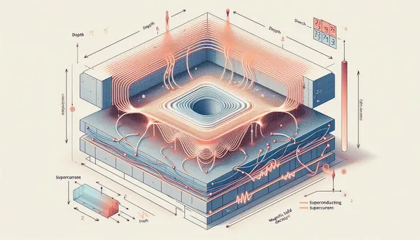
This implies that magnetic fields decay exponentially inside superconductors, instead of persisting like in normal metals. This decay is characterized by the London penetration depth $\lambda_L$ .

📏 London Penetration Depth

Solving Maxwell’s equations with the second London equation gives us:

B(x) = B_0 \, e^{-x/\lambda_L}

Where:

$x$ : Depth into the superconductor
$\lambda_L$ : Penetration depth

Typical values:

For Type I superconductors: $\lambda_L \sim 50 – 500 \, \text{nm}$

📌 This explains the Meissner effect — the magnetic field doesn’t vanish instantly at the surface but decays over a very short distance.

🔄 How Are the London Equations Used?

The London equations are not derived from first principles but are phenomenological — they fit observations.

They help:

Explain magnetic field exclusion
Quantify supercurrent response to electric and magnetic fields
Predict electrodynamic behavior in superconducting wires, films, and devices

📡 Limitations of the London Theory

Despite its usefulness, the London theory has limitations:

No explanation for the origin of superconductivity (unlike BCS theory)
Ignores quantum phase coherence and microscopic interactions
Cannot describe the vortex states in Type II superconductors

📚 Later theories like Ginzburg–Landau and BCS build on the London model and correct these shortcomings.

🧠 Conceptual Summary

Supercurrents in superconductors are non-dissipative, accelerated by electric fields.
Magnetic fields decay exponentially inside, over a scale $\lambda_L$ .
The London equations formalize these behaviors, explaining zero resistance and magnetic field expulsion.

🔮 Coming Up Next…

In Part 7, we’ll explore the Ginzburg–Landau theory — a macroscopic quantum approach to superconductivity. We’ll introduce the order parameter, derive the GL differential equations, and explain how they connect to both Type I/II classification and real-world superconducting phenomena.